

Removing
Motion Blur with Space-Time Processing
Hiroyuki
Takeda and Peyman Milanfar
Although spatial deblurring is relatively well-understood by assuming that the blur kernel is shift-invariant, motion blur is not so when we attempt to deconvolve this motion blur on a frame-by-frame basis: this is because, in general, video include complex, multi-layer transitions. Indeed, we face an exceedingly difficult problem in motion deblurring of a single frame when the scene contains motion occlusions.
Instead of deblurring video frames, individually, a fully 3-D deblurring method is proposed in this work to reduce motion blur from a single motion-blurred video to produce a high resolution video in both space and time. The blur kernel is free from explicit knowledge of local motions unlike other existing motion-based deblurring approaches. Most importantly, due to its inherent locally adaptive nature, the 3-D deblurring is capable of automatically deblurring the portions of the sequence which are motion blurred, without segmentation, and without adversely affecting the rest of the spatiotemporal domain where such blur is not present.
Our proposed approach is a two-step approach: first we upscale the input video in space and time without explicit estimates of local motions and then perform 3-D deblurring to obtain the restored sequence.
Extra Examples
1. Rotation
This example shows that the temporal deblurring of video
effectively removes non-uniform motion blur effects without segmentation
or local motion information. In this example, we compare our deblurring
method in the space-time domain to Fergus' and Shan's blind deblurring
methods in the spatial domain. In the current implementations of those
two blind methods, the PSF is assumed to be a shift-invariant.
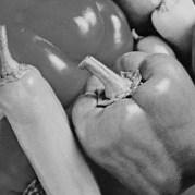
Using the rotating pepper video, generated by rotating a still pepper image counterclockwise 1 degree per frame (shown at the left in Fig.1(f) below), we created a non-uniform motion blur video by blurring the original rotating video with a temporal (shift-invariant 1x1x8) uniform PSF. The resulting video is shown at the center in Fig.1(f). The motion blur can be caused by the rotation of the camera. The motion deblurred frame by Fergus' and Shan's methods are shown in Fig.1(c) and (d), respectively, with their estimated spatial PSFs. Due to the non-uniform blur, the underlying spatial PSF would be shift-variant. However, for videos, simply deblurring the motion blurred video with the 1x1x8 shift-invariant can remove the non-uniform motion blur effectively as shown in Fig1.(e) and the right of Fig1.(f).
The simulation program is available here.
 |
||
(a)
A frame from the original rotating video |
(b)
A frame from a blurred video PSNR = 27.10[dB] |
|
 |
||
(c)
Fergus' method PSNR = 23.23[dB] |
(d)
Shan's method PSNR = 25.18[dB] |
(e)
our 3-D deblurring PSNR = 33.12[dB] |
 |
(f)
the rotating videos: (left) the original, (center) the blurred video,
(right) our deblurred video. |
2.
Global Shift
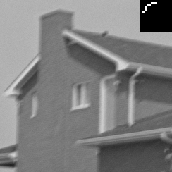
The second example is another motion deblurring, where the
motion blur is uniform in one frame, but different in each frame. We created
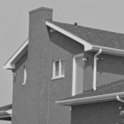
a sequence by circularly shifting a still house image. The resulting video
is shown in the left of Fig.2(g), and one frame of the video is shown
in Fig.2(a). Similar to the rotation example above, we blur the house
video with a 1x1x8 (temporal) uniform PSF, and add white Gaussian noise
to the blurred video (STD = 2). The simulated blurry and noisy video is
shown in the center of Fig.2(g). Since the motion is pure translational
in this example, knowing the spatial displacements between frames (or
motion vectors) and the exposure time (i.e. 8-frame-length), we can easily
compute the equivalent motion PSF in the spatial domain, which are shown
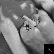
at the upper-right corner of Fig.2(b) and in Fig.2(g).
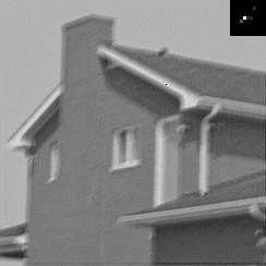
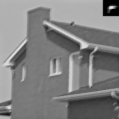
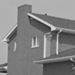
When the motion PSF is known, we can simply deblur the frames with the motion PSF. The deblurred frames with 2-D total variation in the spatial domain is shown in Fig.2(c). If the underlying motion PSF is unknown, the blind deconvolution method is one option. The deblurred results by the blind methods of Fergus et al. and Shan et al. are shown in Fig.2(d) and (e), respectively. The estimated PSFs are also shown at the upper-right corners. However, for video, we can remove the motion blur from the video by deblurring with a shift-invariant 1x1x8 uniform PSF without motion information or estimation of a motion PSF for each frame. Our deblurred frames in the space-time domain are shown at the right in Fig.2(g).
The simulation program is available here.
 |
 |
 |
(a)
A frame from the original rotating video |
(b)
A frame from a blurred video PSNR = 28.22[dB] |
(c)
The deblurred frame in the spatial domain with the true 2-D PSF
and 2-D TV |
 |
 |
 |
(d)
Fergus' method PSNR = 27.79[dB] |
(e)
Shan's method PSNR = 28.68[dB] |
(f)
our 3-D deblurring PSNR = 34.70[dB] |
 |
(g)
the original videos: (left) the original, (center) the blurred video,
(right) our deblurred video. |
3. Motion
Deblurring with Different Temporal Upscaling Factors
This
simulation shows how the choice of the temporal upscaling factor (the
factor of the frame-rate upconversion) affects our deblurring results.
First we create an high resolution, high speed video of the UC seal image by horizontal shifting, where the maximum motion speed is 1 pixel per frame. Let the frame rate of the video be 8 fps (frame per second) for convenience, and the video is shown in Fig.3(a) below. Next, suppose we shoot the moving UC seal using a low speed video camera at 1fps with the exposure time 1 second. This yields us a blurry low speed video at 1 fps shown in Fig.3(b), which is equivalently given by blurring the high speed video of Fig.3(a) with a 1x1x8 uniform (temporal) PSF and, then, temporally downsampling the blurred video with the factor of 8:1 (no noise is added).
The first step of our deblurring approach is to increase the frame rate of the low speed video. In this simulation, in order to see the difference of the deblurred results, instead of estimating the intermediate frames by the space-time interpolation, we insert true intermediate frames to the low speed video to increase the frame rate. By this, we simulated three upscaled videos at different frame rates, 2fps, 4fps, and 8fps, which are shown in Figs.3(c), (d), and (e), respectively.
The final step is to deblur the simulated upscaled videos. Since the exposure time is 1 second, we select the temporal PSF 1x1x2, 1x1x4, 1x1x8 uniform for Figs.3(c), (d), and (e), respectively. Using the PSFs, we deblur the upscaled videos with 3-D total variation regularization and the same regularization parameter. The deblurred videos of Figs.3(c), (d), and (e) are shown in Figs.3(f), (g), and (h), respectively. As seen in the results, the higher the temporal upscaling factor is, we can reduce the motion blur the more effectively. However, we select the temporal upscaling factor not by the amount of motion blur, but the desired frame rate.
The simulation program is available here.
 |
|||
|
|||
 |
|||
|
|||
 |
|||
|
4. Vent
Example
The
last example is a real deblurring example of Vent sequence shot by Shechtman
et al. where a fan is revolving very fast. The sequence is available
here.
The space-time superresolution method proposed by Shechtmanet al. uses
4 videos taken by 4 cameras at the same time with slight spatial and temporal
displacements, and fuse them together to increase the spatial and temporal
resolution. A post-process was carried out to remove the spatial blur
and temporal (motion) blur.
However, the fan is revolving so fast that the fan blades are still motion-blurred as shown in Figs.4(a) and (b). In this example, we use Shechtman's space-time superresolved Vent video as our low speed video, and reduce the motion blur further. We temporally upscale the vent video with the upscaling factor 8 (after upscaling, the frame rate of our upscaled video is 8 times faster than Shechtman's superresolved video), and deblur the upscaled video with a 1x1x12 uniform PSF. We note that the temporal support of the PSF is larger than the upscaling factor probably because the effective exposure time of Shechtman's output video is longer than the frame interval.
 |
 |
 |
 |
(a)
Shechtman's space-time superresolution (t=61) |
(b)
Our deblurred result (t = 61) |
(c)Shechtman's
space-time superresolution (t=62) |
(d)
Our deblurred result (t=62) |
Acknowledgements
This work was supported in part by the US Air Force Grant FA9550-07-1-0365 and the National Science Foundation Grant CCF-1016018.