VEES Tutorial, version 0.0.1e

Table of contents

Windows setup using vees zoom and rotate exploring/filtering data adjusting the color map Time step record/playback

Windows setup:

1. Place OpenSees.exe in the same folder with glut32.dll, glui32.lib and your tcl scripts
2. Modify your tcl scripts by adding the command, vees
   The vees command does not get loaded into OpenSees until after the model is declared, e.g.
   
   model BasicBuilder -ndm 3 -ndf 3
   
   Calling vees should then give you the graphical user interface, but to see your mesh, call vees after creating your nodes and elements. Note: when vees closes it will also close OpenSees.exe (a bug!)
3. Click OpenSees.exe to start. When your script reaches the vees command it will open 2 windows

Using VEES:

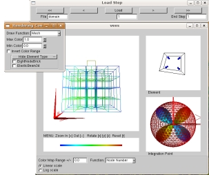
In any of the vees display windows, you can interact by placing the mouse in the display window and using the following keyboard commands:

• [x] rotate about x axis
• [y] rotate about y axis
• [z] rotate about z axis
• [+] zoom in
• [-] zoom out
• [r] reset to original orientation

Clicking an eight node brick will show its gauss integration points.

In the rendering control window you can choose from a drop down menu of drawing methods. 20 node bricks have not yet been implemented.

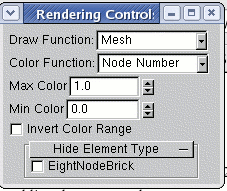
You can select from several coloring schemes. Each is scaled into into a 0 to 1 range, where 0 is blue, 0.5 is green, 1 is red.

• By element type assigns each element type a unique random color.
• By displacement sums the absolute values from each degree of freedom up to the number of dimensions of the node (2 or 3)

There are two types of filters to explore the data:

• By value: you can limit the upper and lower value using the Max Color and Min Color spinners, and also invert the range (show everything outside the selected range)
• By element type: check the box for the element type you would like to hide.
  

 
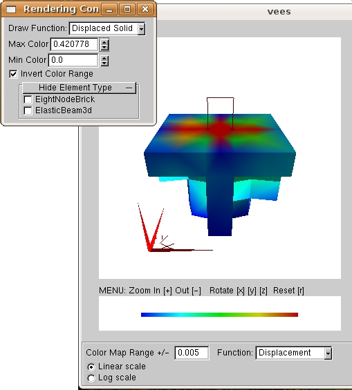
Color map range adjustment:
At the bottom, there is a a new widget set for color maps. You can select the color map from the drop down list. The range for the color map is set to the (absolute) maximum for the time step at which you called vees. If the vales for the time step are all very small (absolute value between 0 and 1.0) the the color map range max is set to 1.0

You can adjust the color map range by clicking on the text area, using the backspace key to remove old digits and then typing in new ones. Sometimes it sticks a little, just click another part of the interface and click back to make it work.

Time step record/playback:

I have added a new recorder that records all node data (degrees of freedom, etc.) and stress, strain, and stiffness for many elements and materials. The command is

recorder domain <-file $filename>

Specifying the file name is optional. The default file names will be domain1, domain2, etc. Be careful, the files can be quite large for the 3D soil materials.

The files can then be reloaded using the new widget shown below:

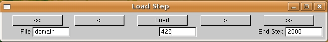
You can load a specific time step by entering the step number in the text area under the load button and clicking Load.
To move to the next time step, click the '>' button. Use the '<' button to load the previous step.

To run through many time steps as a movie, enter the first time step in the text area below the Load button and the
last time step in the text area labeled End Step. Then click the '>>' button to run forward, or '<<' to run backwards.

I find it useful to load the last  time step,  set the color map ranges, and then run through the time steps as a movie.